Sentiment analysis is a common task in natural language processing. Many of the tools available for this are calibrated to the English language. Can Google Translate let us apply this toolset to a broader set of languages? We will use the tidytext framework to measure sentiment of tweets originally in African languages but translated to English. We’ll measure sentiment at both the word level and sentence level and see how it agrees with the sentiment, positive, negative or neutral, already assigned in the Afrisenti data set.
In Our Last Episode…
In part one of this series we translated the afrisenti data set using the Google Cloud Translate API. This data set contains a little over 110,000 tweets in 13 different African languages(Muhammad et al. 2023). We saw that , at first glance, Google Translate does a good job on these languages. So now let’s ask:
Are the translations good enough to run sentiment analysis on?
Will the sentiments we measure agree with the original data? This is a higher standard, of course.
Measuring Sentiment
Now that we have all of the tweets translated into English we can use sentiment tools calibrated to the English language. We will try two different approaches. For both we’ll compare the measured sentiment of the English tweet to the assigned sentiment in the data set.
Measure the sentiment “valence” of each word as either positive or negative and take the balance of positive vs. negative as the sentiment of the tweet.
Negation turns a positive sentiment into a negative one. “I do not like” has one positive word, “like,” but is clearly a negative sentiment. Rather than measure each word, we can run a sentence-level model to see if we get a better result.
First load the needed packages and the translated tweets from part one of this project.
#load librariessuppressPackageStartupMessages({library(tidyverse)library(tidytext)library(hunspell)library(sentimentr)library(magrittr)})# set up some chart defaultstan1 <-"#FDECCD"yellow1 <-"#FFBF00"green1 <-"#007000"theme_afri <-function(...){# making a function allows passing further theme elements ggplot2::theme(plot.background =element_rect(fill = tan1, color =NA),panel.background =element_blank(),legend.background =element_blank(),legend.box.background =element_blank(),legend.key =element_blank(), ... ) }afrisenti_translated <- readr::read_csv('https://raw.githubusercontent.com/apsteinmetz/tidytuesday/master/2023-02-28_african_language/data/afrisenti_translated.csv',show_col_types =FALSE) |>select(tweet_num,assigned_long,translatedText,label) |>mutate(label =as.factor(label))afrisenti_translated
# A tibble: 111,720 × 4
   tweet_num assigned_long translatedText                                  label
       <dbl> <chr>         <chr>                                           <fct>
 1         1 Amharic       Amhara region needs moderation!!! He hates Mus… nega…
 2         2 Amharic       Having a mood in a way that annoys someone....  nega…
 3         3 Amharic       Domestic violence - without hearing - without … nega…
 4         4 Amharic       Ethiopia, what was your role in overthrowing T… nega…
 5         5 Amharic       No matter how Oromo learns, they don't realize… nega…
 6         6 Amharic       Tish, dark powder, are you standing at 97? Tim… nega…
 7         7 Amharic       Local residents said that the internet and tel… nega…
 8         8 Amharic       What happened to Schimmels is sad. By the word… nega…
 9         9 Amharic       An unstable country does not need elections     nega…
10        10 Amharic       The idiot and the bubble, the Ethiopian PM Abi… nega…
# ℹ 111,710 more rows
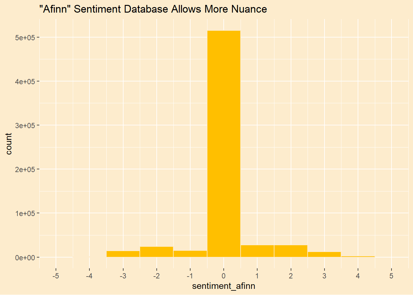
The tidytext package makes it easy to divide each tweet into separate words and measure the sentiment valence of each one. The tidytext package has a few sentiment lexicons. Here, we decide the sentiment of each word using the “afinn” lexicon. We chose this because it has 11 shades of sentiment and we hope the finer granularity will be helpful. If a word is not in the lexicon we code it as”0” or neutral. Further, we need to use the stems of words. “Idiots” is not in our sentiment sources, “Idiot” is. Word stemming will fix that. The hunspell package using hunspell_stem() will do the trick. It returns a list of possible stems (usually just one, but not always) so we have to unnest() the list column. The trade-off is that if the word is not in hunspell’s dictionary, it drops the word. Fortunately, there are over 49,000 words in the dictionary.
I don’t know who decided that “superb” gets a “+5” and “euphoric” gets a “+4,” but there you are. We can see how the valences are distributed in our tweets. The vast majority of words are not in the lexicon and therefore are coded as zero, neutral.
# A tibble: 5 × 2
  word       sentiment_afinn
  <chr>                <dbl>
1 idiot                   -3
2 cannibal                 0
3 forgivable               0
4 renegade                 0
5 people                   0
The benefits and drawbacks of stemming are apparent. We can find the stem of “idiots” and “cannibals” but “unforgivable” gets changed to “forgivable” which flips its sentiment. No matter because neither word is in our sentiment lexicon. There are no positive words in this tweet so the sum of all the valences is negative, which matches with the assigned sentiment.
Next we add up the valences for each tweet to arrive at the net sentiment.
tweet_sentiment <- tweet_word_sentiment %>%group_by(tweet_num) %>%summarise(sentiment_afinn =as.integer(sum(sentiment_afinn))) %>%ungroup() |>full_join(afrisenti_translated,by =join_by(tweet_num)) |>mutate(language =as_factor(assigned_long)) |>rename(label_original = label) |># set NA sentiment to neutralmutate(across(contains("sentiment"),~replace_na(.x,0)))
We have numeric valences. If we want to compare our measurment to the original we have to make a choice what to label each number. Obviously, zero is neutral but should we expand the neutral range to include, say -1 and +1? Sadly, no. The summary below shows that we already assigned far more neutral labels than the original data set has. This is not a good omen. We wish we had more granularity.
# A tibble: 10 × 2
   label_original translatedText
   <fct>          <chr>
 1 positive       "@user Amen Thanks so much fam... God bless you all"
 2 neutral        "No need to extend us. https://t.co/cKIft7Aqk5"
 3 positive       "Our king is one Mohammed VI... Long live the king and long l…
 4 positive       "'@user @user @user @user and every time the son of their mou…
 5 positive       "@user This problem of insecurity that we are dealing with ma…
 6 positive       "Just as our bodies have a great need for food, so even our h…
 7 neutral        "RT @user: You definitely can improve your #yoruba by watchin…
 8 positive       "@user Tanemi forgiveness and forgiveness, God is the best, G…
 9 positive       "@user Don't agree! We want him to continue as president beca…
10 negative       "This is the appropriate response that deserves the likes of …
Our scoring looks pretty good. Where we disagree with Afrisenti, I side with tidytext for the most part. Having said that, the provided sentiments are human-curated with at least 2 out of 3 native language speakers agreeing on how to code each tweet. So who am I to argue?
Here are samples of negative-scored tweets with along the original sentiment.
# A tibble: 10 × 2
   label_original translatedText
   <fct>          <chr>
 1 positive       "@user Good man, this time is up. The children and the childr…
 2 neutral        "who died in power"
 3 positive       "SAY NO TO SUICIDE!!! Reposted from @user - We have some tips…
 4 negative       "Hunger has no respect \U0001fae1"
 5 negative       "@user And you started ruining it with lies \U0001f914\U0001f…
 6 positive       "@user @user @user @user @user @user God forbid evil!"
 7 neutral        "'It's father Kashi, you can leave this beautifully and go ho…
 8 neutral        "Tete provincial finance director arrested https://t.co/guJWN…
 9 negative       "@user Just as Barcelona were tired, PSG will also be tired, …
10 negative       "u see diz life e no go make u hype somethings see diz otondo…
It’s the same story with the negative tweets. We do a reasonable job and the correctness of the original sentiment is arguable. There is a lot of disagreement.
We can generate a confusion matrix with some additional statistics to look at the agreement of our measurements vs. the human classifiers. Ideally all the observations would lie on the diagonal from top left to bottom right.
# A tibble: 2 × 6
  term     class estimate conf.low conf.high    p.value
  <chr>    <chr>    <dbl>    <dbl>     <dbl>      <dbl>
1 accuracy <NA>     0.511    0.509     0.514  2.58e-234
2 kappa    <NA>     0.264   NA        NA     NA
It’s not me, it’s you.
As we look at the cross-tab there are many, many incorrect classifications. The accuracy for both of these measures is scarcely more that 50%. The “Kappa” statistic shows that we are only about 26% better than random chance. It’s not zero but it’s not good. Why the disappointing result? First of all, our valence measure isn’t opinionated enough. There are far too many neutral tweets.
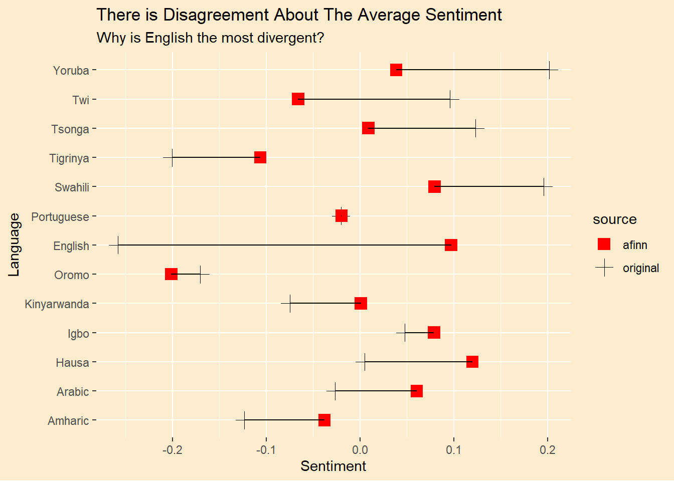
avgs <- tweet_sentiment |>group_by(language) |>summarise(across(contains("label"),~mean(as.numeric(.x)-2),.names ="mean_{str_remove(.col,'label_')}")) |>pivot_longer(cols =contains("mean"), names_to ="source",values_to ="average") |>mutate(source =str_remove(source,"mean_"))# plot the sentiment distribution by languageavgs |>ggplot(aes(y = average,x = language)) +geom_point(aes(color = source,shape = source),size =4) +geom_line() +scale_y_continuous(n.breaks =5) +scale_shape_manual(values =c(afinn =15,sentence=19,original =3)) +scale_color_manual(values =c(afinn ="red",sentence=green1,original ="black")) +scale_fill_manual(values =c(afinn ="red",sentence=green1,original ="black")) +theme_afri() +labs(y="Sentiment",x="Language",title ="There is Disagreement About The Average Sentiment",subtitle ="Why is English the most divergent?") + ggplot2::coord_flip()
You may wonder if one of the other sentiment lexicons would produce a better result. I have tried the others but I don’t include them here because the results are substantially identical.
In our defense, I’m not sure the Afrisenti sentiment assignments are better, as we saw above. But maybe that just means Google Translate has stripped some of the emotion out of them that is present in the original language. I don’t know, but this would mean Google Cloud Translate doesn’t work for this purpose.
Here’s the puzzle, though. The biggest disagreement about sentiment is in English-language tweets, where no translation is needed so we can’t blame Google for this. A look at some English tweets reveals that they are mostly in Pidgin so the vocabulary is not what we would expect in the sentiment sources we’re using. Here are some random English tweets:
# A tibble: 5 × 1
  translatedText
  <chr>
1 jesus taught i had sef
2 better all those figures they are generating if u never dey vex reach na the …
3 people don dey find themselves from twitter oo and that ilorin where everyone…
4 it's sweet soul abeg
5 as a guyman used to paying the lump sum and calling it a day with the mindset…
So, paradoxically, the translated tweets of truly foreign languages are rendered into more standard English.
Maybe we’ll get more agreement if we address negation, as mentioned above. The tweet below illustrates the problem.
afrisenti_translated$translatedText[28670]
[1] "@user Why don't America want the world to be peaceful 🤔🤔🤔"
# A tibble: 3 × 4
  tweet_num label    word     sentiment_afinn
      <dbl> <fct>    <chr>              <dbl>
1     28670 negative user                   0
2     28670 negative world                  0
3     28670 negative peaceful               2
Unless the negation is itself a negative valence word, many negative tweets will test as positive. In this example “peaceful” is positive but “don’t want” clearly flips it.
A More Sophisticated Approach
There are a number of approaches to solve the negation problem. A simple one is to combine negation words like “no” and “not” with the subsequent one. We will use this approach in our next post attempting machine learning. Here we’ll try sentence-level measurement using the sentimentr package. This package understands negation better. Our test tweet from above is a challenge. This is since the negation of “peaceful” comes eight words before “not.” The default of n.before = 5 doesn’t give us the right answer.
mytweets <-"Why don't America want the world to be peaceful"sentimentr::sentiment(mytweets,n.before =5)
As before, we start by breaking the tweets up into constituent parts, sentences in this case. Most tweets will be just one sentence of course. Again we compute a sentiment score, this time with the sentiment_by() function. It yields a finer grained sentiment score than our earlier measures.
I am using a less common pipe operator below, %$% from the magrittr package, which expands the list-column created by get_sentences. Normally I would use tidyr::unnest() to do this but it loses the special object class that sentiment_by() needs. The sentimentr package uses the fast data.table vernacular, not the dplyr one, which I mostly use here.
Before we look at the tweet-level sentiment let’s group by language. This lets us see if the sentiment measure is consistent across languages.
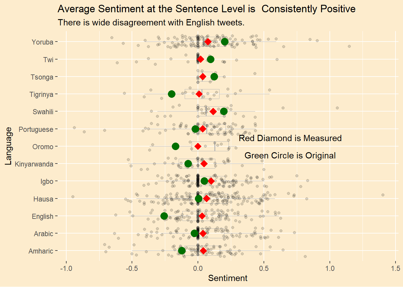
avgs <- tweet_sentence |>group_by(language) |>summarise(ave_sentiment =mean(ave_sentiment))avgs_orig <- afrisenti_translated |>group_by(assigned_long) |>summarise(ave_sentiment =mean(as.numeric(label)-2))# plot the sentiment distribution by languagetweet_sentence |>as_tibble() |># make the size manageableslice_sample(n=1000) |>group_by(language) |>rename(sentiment = ave_sentiment) |>ggplot() +geom_boxplot(aes(y = sentiment, x = language),fill =NA,color ="grey70",width =0.55,size =0.35,outlier.color =NA ) +geom_jitter(aes(y = sentiment, x = language),width =0.35,height =0,alpha =0.15,size =1.5 ) +scale_y_continuous(n.breaks =5) +# theme_bw() +theme_afri() +geom_point(data = avgs,aes(y = ave_sentiment, x = language),colour ="red",shape =18,size =4) +geom_point(data = avgs_orig,aes(y = ave_sentiment, x = assigned_long),colour = green1,shape =19,size =4) +ylab("Sentiment") +xlab("Language") +labs(title ="Average Sentiment at the Sentence Level is Consistently Positive",subtitle ="There is wide disagreement with English tweets.") +annotate("text",y = .7,x=7.5,label ="Red Diamond is Measured") +annotate("text",y = .7,x=6.5,label ="Green Circle is Original") +coord_flip()
The dots are the measured sentiment of a sample of tweets. The markers are the average measured sentiment (red diamond) and average original sentiment (green circle), across all tweets. The measured sentiment looks more consistent then the original. The tweets in all languages are scored, on average, positive, by our calculations. We obviously disagree with the original. Note that the original 3-level sentiment as been converted to a numeric range, -1 to 1, to compute the green markers, whereas the range for our measurements is much wider.
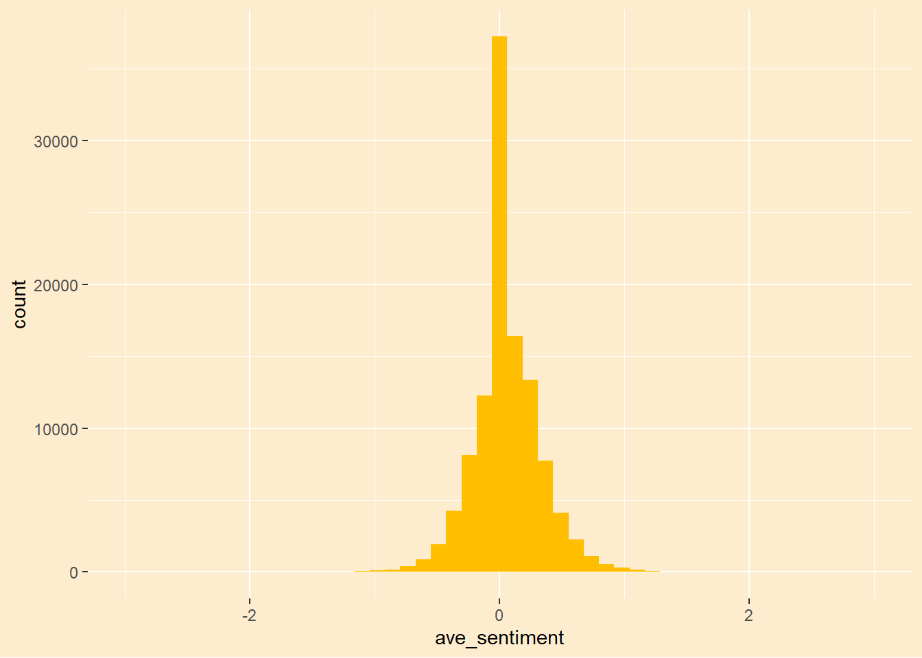
We no longer have the problem where too many tweets are neutral. The median of the distribution above is zero but there are far fewer tweets that are of exactly zero valence. This let’s us expand the range of neutral above and below zero. I tried to balance the data to match the distribution of sentiment in the original data as closely as possible.
While we’re at it let’s put our results together.
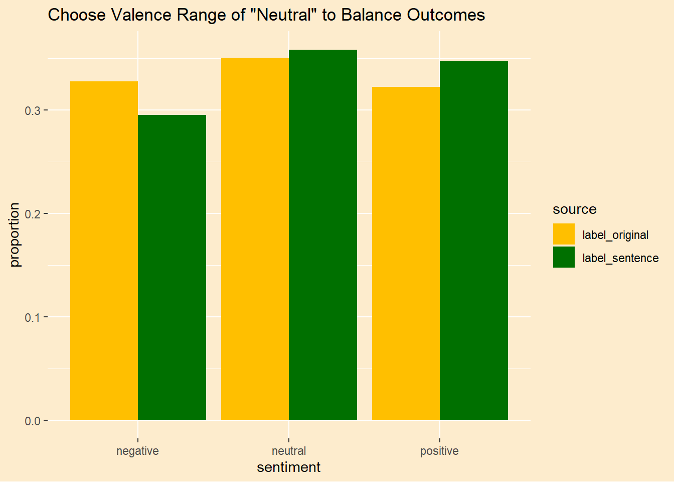
# picked these levels to balance the data setlow =-0.01high =0.12tweet_sentence <- tweet_sentence |>as_tibble() |>mutate(label_sentence =cut(ave_sentiment,breaks =c( -Inf,low,high,Inf), labels=c("negative","neutral","positive")))tweet_sentiment <-left_join(tweet_sentiment, tweet_sentence,by =join_by(language, tweet_num))
Compare our distribution to the original.
tweet_sentiment |>pivot_longer(c(label_original,label_sentence),names_to ="source",values_to ="sentiment") |>group_by(source,sentiment) |>count() |>group_by(source) |>reframe(sentiment,proportion = n/sum(n)) |>ungroup() |>ggplot(aes(sentiment,proportion,fill=source)) +geom_col(position ="dodge") +scale_fill_manual(values =c(yellow1,green1)) +theme_afri() +labs(title ='Choose Valence Range of "Neutral" to Balance Outcomes')
A Dissapointing Outcome
As you can see, we are pretty balanced. This is kind of cheating because we are calibrating the category breakpoints to the known data. We should be calibrating to a training set and then see how it works on the test set. Let’s just see if the in-sample fit is any good first.
# A tibble: 2 × 6
  term     class estimate conf.low conf.high p.value
  <chr>    <chr>    <dbl>    <dbl>     <dbl>   <dbl>
1 accuracy <NA>     0.510    0.507     0.513       0
2 kappa    <NA>     0.265   NA        NA          NA
Wow. That’s disappointing. The agreement with the original sentiment is nearly identical to the word-level measurements. That is, poor. I thought balancing the outcomes to match the frequency of the original would help, at least.
# A tibble: 2 × 6
  term     class estimate conf.low conf.high p.value
  <chr>    <chr>    <dbl>    <dbl>     <dbl>   <dbl>
1 accuracy <NA>     0.620    0.617     0.623       0
2 kappa    <NA>     0.425   NA        NA          NA
Conclusion
If we take the sentiment labels in the original data set as “true,” our sentiment valence measurements in English do a poor job. A cursory visual examination reveals that the sentiment we assigned with our valence measures look pretty reasonable in most cases but do not predict what is in the Afrisenti data set very well. We therefore conclude that Google Cloud Translate doesn’t match well with these tweets using tidytext methods.
We’re not defeated yet. Our measurements had no knowledge of what the original sentiments were. What if we could learn the inscrutable methods used to assign sentiment in the original? In the next post we’ll apply machine learning to see if we can train a model using the translated tweets that is in closer agreement with the Afrisenti data set.
References
Muhammad, Shamsuddeen Hassan, Idris Abdulmumin, Abinew Ali Ayele, Nedjma Ousidhoum, David Ifeoluwa Adelani, Seid Muhie Yimam, Ibrahim Sa’id Ahmad, et al. 2023. “AfriSenti: A Twitter Sentiment Analysis Benchmark for African Languages.” In.
Silge, Julia, and David Robinson. 2016. “Tidytext: Text Mining and Analysis Using Tidy Data Principles in r.”The Journal of Open Source Software 1 (3): 37. https://doi.org/10.21105/joss.00037.